MobileNetV2: Inverted Residuals and Linear Bottlenecks - Mark Sandler Andrew Howard Menglong Zhu Andrey Zhmoginov Liang-Chieh Chen Google Inc.
이번 포스팅에서는 구글에서 발표한 Mobilenet v1에 이어서 Mobilenet v2(2018)에 대해 살펴보려고 한다. Mobilenet v1에서의 핵심 아이디어인 Depthwise separable convolution을 역시 그대로 사용하되 Inverted Residual 구조를 제시하였다.
1. What has changed?

Mobilenet v1
- 일반적인 Convolution구조를 Depthwise separable convolution로 바꾸어서 3x3 filter를 사용하였을때 약 8~9배의 연산량을 감소시켰다.
Mobilenet v2
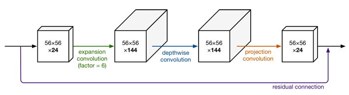
- ResNet의 일반적인 residual learning방법을 사용하지않고 그 반대로 오히려 feature_map의 channel을 확장시킨 후에 Depthwise convolution + pointwise convolution을 수행을 하였다. (그래서 이름이 inverted residual이라고 붙여짐) 그냥 겉으로 보기에는 연산량이 더 증가한 것처럼 보일수 있지만 실제로는 v1보다 연산량이 더 감소하게된다.
- 그리고 Stride 2일때와 1일때 두가지 상황이 존재하는데 v2에서는 stride가 1일때만 skip connection을 하였고 stride 2일때는 단순히 feature size를 절반으로 줄이는 일을 한다. stride가 2일때 skip connection을 하기위해선 input feature size와 동일해야 하기때문에 여기에서 또다른 연산이 필요하기 떄문에 논문에서는 stride가 1일때만 skip connection을 사용하도록 하였다.
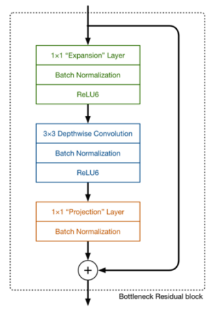
위 사진을 보면 우리가 알고있는 ReLU가 아닌 ReLU6라는것이 사용이 되었는데 ReLU6에 대한 자세한 설명은 아래 링크를 참조하면 좋을 것 같다.
위 그림처럼 inverted residual 구조에서는 블록의 처음 pointwise연산에서 feature의 channel을 확장하는데 논문에서는 t라는 것을 사용해 channel을 확장시켰는데 이것을 expansion factor라고 부른다. t의 배수만큼 channel을 확장시키는데 실험결과 일반적으로 t는 5~10사이가 괜찮았고 그중 6을 택해서 모든 t를 6으로 사용하였다.
2. Inverted Residuals
Inverted Residual에 대해 조금 더 자세히 알아보려고한다. 보통 일반적인 Resdual block은 아래와 같다.
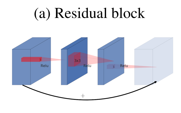
- Residual block은 wide - narrow - wide 한 형태를 띄고 있다.
- network가 진행될수록 보통 channel수(filter 수)가 계속해서 증가하기 때문에 연산량을 절감하기위해 중간에서 1x1 conv로 채널을 한번 줄여준 뒤에 3x3 conv 연산을 하고 다시 원래의 채널로 돌려놓아 skip connection까지 하는 구조이다.
Mobilenet v2에서 제시하는 Inverted Residual 구조는 아래와 같다.
- Inverted Residual block은 일반적인 Residual block과는 정 반대인 narrow - wide - narrow한 형태를 하고있다.
- 이렇게 시도를 한 이유는 narrow에 해당하는 저차원의 layer에는 필요한 정보만 압축되어서 저장되어 있다라는 가정으로부터 나왔다. 따라서 필요한 정보는 narrow에 있기 때문에, skip connection으로 사용해도 필요한 정보를 더 깊은 layer까지 전달할 것이라는 기대를 할 수 있다.
- 그림에서 양끝 레이어가 빗금이 쳐져있는데 이것은 linear bottleneck을 의미하며 즉 Relu를 사용하지 않는다는 것을 말한다. (그 이유는 아래 Linear Bottleneck에 나옴)
- 결과적인 주 목적은 연산량을 감소하기 위함이다.
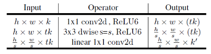
위 사진을 다시 가져와서 연산량이 정말로 줄어드는지 한번 계산해보자.
Input의 크기 : h x w -> 10 x10
Expansion factor : t -> 6
Kernel size : c -> 3
Input channel : t x k -> 6 x 8 = 48
Output channel : t x k' -> 6 x 16 = 96
Movilenet v2
h x w x t x k x 1 x 1 x k + h x w x t x k x c x c x 1 + h x w x k' x 1 x 1 x t x k = h x w x k x t x (k + c^2 + k')
= 10 x 10 x 6 x 8 x (8 + 9 + 16) = 158400
- 위 식에서 빨간색은 각 layer의 output을 의미하고 연두색은 그 output을 계산하기 위한 convolution filter size를 의미한다.
- 첫번째 레이어에서는 pw 연산을 위해 1x1 convolution을 하기 때문에 input channel만 곱해진다.
- 두번째 레이어에서는 dw 연산을 위해 3x3 convolution을 하기 때문에 c x c가 곱해지고 대신 곱해지는 채널의 수가 1이므로 채널은 생략.
- 세번째 레이어는 첫번째 레이어와 동일한 방식이고 연산결과 output channel k'가 나오게 된다.
일반적인 Convolution 및 Mobilenet v1의 연산량과 비교해보면
Simple Convolution
h x w x t x k x c x c x t x k'
= 10 x 10 x 6 x 8 x 3 x 3 x 6 x 16 = 4147200
Movilenet v1
h x w x t x k x c x c x 1 + h x w x t x k' x 1 x 1 x t x k = h x w x k x t x (c^2 + t x k')
= 10 x 10 x 6 x 8 x (9 + 96) = 504000
계산된 feature_map 기준에서 보면 연산량이 일반적인 convolution보다 26배 적고 mobilenet v1보다 3배정도 더 적은것을 확인할 수 있다.
3. Linear Bottlenecks
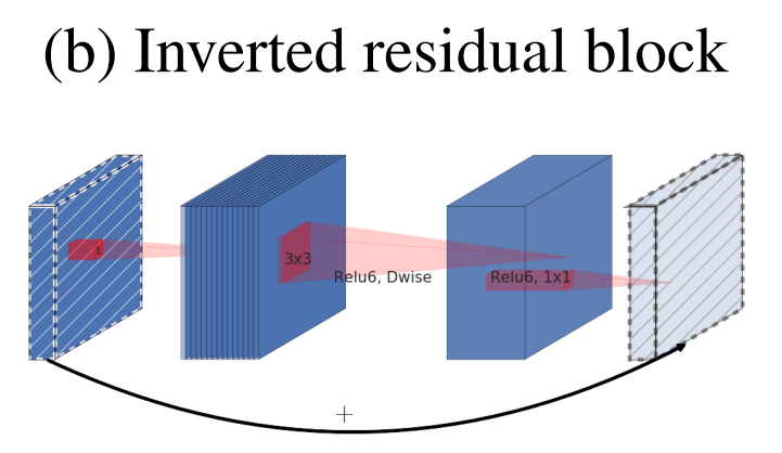
Neural network들은 일반적으로 고차원에서 저차원으로 압축하는 Encoder역할의 네트워크 부분이 발생하고 이 과정에서 feature extraction을 수행하게 된다.
- 위 그림처럼 고차원의 데이터가 저차원으로 압축되면서 특정 정보들이 저차원의 어떤 영역으로 매핑이 되게 되는데, 이것을 manifold라고 이해하면 좋을것 같다.
- 따라서 뉴럴 네트워크의 manifold는 저차원의 subspace로 매핑이 가능하다고 가정을 할 수있다.
- 이런 관점에서 보면 어떤 데이터에 관련된 manifold가 ReLU를 통과하고 나서도 입력값이 음수가 아니라서 0이 되지 않은 상태라면, ReLU는 linear transformation 연산을 거친 것이라고 말할 수 있다. 즉, ReLU 식을 보면 알 수 있는것 처럼, identity matrix를 곱한것과 같아서 단순한 linear transformation과 같다고 볼 수 있는 것이다.
- 그리고 네트워크를 거치면서 저차원으로 매핑이 되는 연산이 계속 되는데, 이 때, (인풋의 manifold가 인풋 space의 저차원 subspace에 있다는 가정 하에서) ReLU는 양수의 값은 단순히 그대로 전파하므로 즉, linear transformation이므로, manifold 상의 정보를 그대로 유지 한다고 볼 수 있다.
- 즉, 저차원으로 매핑하는 bottleneck architecture(projection convolution)를 만들 때, linear transformation 역할을 하는 linear bottleneck layer(Don't use ReLU)를 만들어서 차원은 줄이되 manifold 상의 중요한 정보들은 그대로 유지해보자는 것이 컨셉이다.

- ReLU는 0이하의 값을 0으로 만들기때문에 그만큼의 정보손실이 있을수밖에 없다.
- 위 그림에서 볼 수 있듯이 저차원에서의 맵핑 정보손실이 더 크고 그 의미는 ReLU를 차원수가 충분히 큰 공간에서 사용하게 된다면 그만큼 정보 손실율일 낮아진다는 것을 의미한다.
- 여기까지는 가설이지만, 실제로 실험을 하였는데 bottleneck layer를 사용하였을 때, ReLU를 사용하면 아래그림처럼 오히려 성능이 떨어진다는 것을 확인했다고 한다.

논문에서 다음과 같이 설명하고 있다.
1. If the manifold of interest remains non-zero volume after ReLU transformation, it corresponds to a linear transformation.
2. ReLU is capable of preserving complete information about the input manifold, but only if the input manifold lies in a low-dimensional subspace of the input space.
- assuming the manifold of interest is low-dimensional we can capture this by inserting linear bottleneck layers into the convolutional blocks.
그렇기 때문에 아래 그림처럼 Expansion Layer에서는 ReLU6를 사용하지만 Projection Layer에서는 Low-dimension 데이터를 출력하기 때문에 여기에 non-linearity를 사용하게 되면 데이터의 유용한 정보들이 손실된다는 것이 논문의 주장이다.
4. Model Architecture
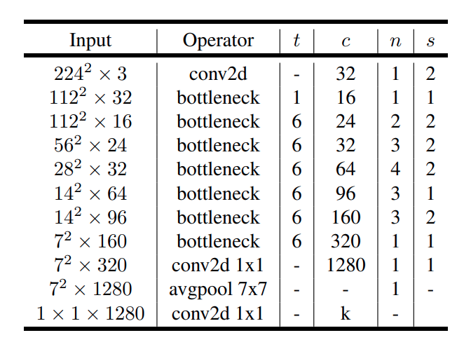
위 사진은 Mobilenet v2의 모델 구조이다. Input size는 Imagenet data로 실험을 했기 때문에 224 x 224 x 3 사이즈이며 최종 k는 1000으로 되어있다. 각 파라미터의 의미는 아래와 같다.
- t = expansion factor
- c = channal
- n = iteration
- s = stride
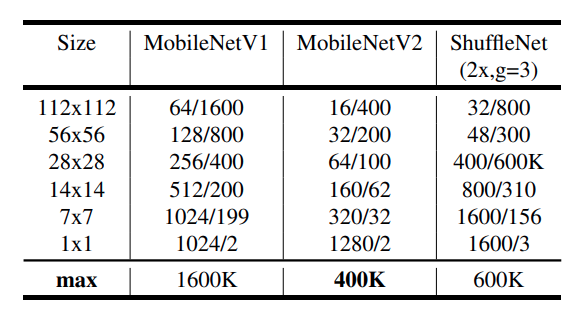
위 사진은 비교적 가벼운 모델들의 각 feature_map에서의 channels/memory 를 보여주는 표이다. 볼 수 있듯이 Mobilenet v2의 채널수가 적고(bottleneck 에서만 expansion시키고 다시 projection하기 때문) 메모리 사용량도 더 적기 때문에 embadded system에 가장 적합하다는 것을 알 수 있다.
Pytorch 구현
데이터는 캐글의 Intel Image Classification이라는 자연 풍경 데이터를 사용하였다.
Download Link - www.kaggle.com/puneet6060/intel-image-classification
Data information
- Class - buildings, forest, glacier, mountain, sea, street
- Image size - 150 x 150 x 3
- Amount - 14k images in Train, 3k in Test and 7k
ImageNet data에 대해 pretrained된 weights를 통해 현재 데이터에 10 epoch으로 Finetuning을 진행하였다.
Model Define
import torch.nn as nn
import math
from torchsummary import summary
import pdb

# 첫번째 layer에서 사용될 convolution 함수
def conv_bn(inp, oup, stride):
    return nn.Sequential(
        nn.Conv2d(inp, oup, 3, stride, 1, bias=False),
        nn.BatchNorm2d(oup),
        nn.ReLU6(inplace=True)
    )

# inverted bottleneck layer 바로 다음에 나오는 convolution에 사용될 함수
def conv_1x1_bn(inp, oup):
    return nn.Sequential(
        nn.Conv2d(inp, oup, 1, 1, 0, bias=False),
        nn.BatchNorm2d(oup),
        nn.ReLU6(inplace=True)
    )

# channel수를 무조건 8로 나누어 떨어지게 만드는 함수
def make_divisible(x, divisible_by=8):
    import numpy as np
    return int(np.ceil(x * 1. / divisible_by) * divisible_by)


class InvertedResidual(nn.Module):

    def __init__(self, inp, oup, stride, expand_ratio):
        super(InvertedResidual,self).__init__()
        self.stride = stride
        assert stride in [1,2]

        hidden_dim = int(inp * expand_ratio)  # expansion channel
        self.use_res_connect = self.stride == 1 and inp == oup  # skip connection이 가능한지 확인 True or False
        '''
        self.stride == 1 ----> 연산 전 후의 feature_map size가 같다는 의미
        inp == oup ----> 채널수도 동일하게 유지된다는 의미
        즉 skip connection 가능
        '''
        if expand_ratio == 1:
            self.conv = nn.Sequential(
                # 확장시킬 필요가 없기 때문에 바로 depth wise conv
                nn.Conv2d(hidden_dim, hidden_dim, 3, stride, 1, groups=hidden_dim, bias=False),
                nn.BatchNorm2d(hidden_dim),
                nn.ReLU6(inplace=True),
                # pw-linear
                nn.Conv2d(hidden_dim, oup, 1, 1, 0, bias=False),
                nn.BatchNorm2d(oup)
            )
        else:
            self.conv = nn.Sequential(
                # pw(확장)
                nn.Conv2d(inp, hidden_dim, 1, 1, 0, bias=False),
                nn.BatchNorm2d(hidden_dim),
                nn.ReLU6(inplace=True),
                # dw
                nn.Conv2d(hidden_dim, hidden_dim, 3, stride, 1, groups=hidden_dim, bias=False),
                nn.BatchNorm2d(hidden_dim),
                nn.ReLU6(inplace=True),
                # pw-linear(축소)
                nn.Conv2d(hidden_dim, oup, 1, 1, 0, bias=False),
                nn.BatchNorm2d(oup)
            )

    def forward(self, x):
        if self.use_res_connect:
            return x + self.conv(x)  # skip connection (element wise sum)
        else:
            return self.conv(x)


class MobileNetV2(nn.Module):

    def __init__(self, n_class=1000, input_size=224, width_mult=1.):
        super(MobileNetV2, self).__init__()
        block = InvertedResidual
        input_channel = 32
        last_channel = 1280

        interverted_residual_setting = [
            # t, c, n, s
            # t : expand ratio
            # c : channel
            # n : Number of iterations
            # s : stride
            [1, 16, 1, 1],
            [6, 24, 2, 2],
            [6, 32, 3, 2],
            [6, 64, 4, 2],
            [6, 96, 3, 1],
            [6, 160, 3, 2],
            [6, 320, 1, 1]
        ]

        # building first layer
        assert input_size % 32 == 0
        # input_channel = make_divisible(input_channel * width_mult)
        self.last_channel = make_divisible(last_channel * width_mult) if width_mult > 1.0 else last_channel
        self.features = [conv_bn(3, input_channel, 2)]  # feature들을 담을 리스트에 first layer 추가

        # building inverted residual blocks
        for t, c, n, s in interverted_residual_setting:
            output_channel = make_divisible(c * width_mult) if t > 1 else c
            for i in range(n):
                if i == 0:
                    self.features.append(block(input_channel, output_channel, s, t))
                else:
                    self.features.append(block(input_channel, output_channel, 1, t))  # 반복되는 부분에서 skip connection 가능
                input_channel = output_channel
        # building last several layers
        self.features.append(conv_1x1_bn(input_channel, self.last_channel))  # (batch, 320, 7, 7) -> (batch, 1280, 7, 7)
        # make it nn.Sequential
        self.features = nn.Sequential(*self.features)

        # Average pooling layer
        self.avg = nn.AvgPool2d(7, 7)
        # building classifier
        self.classifier = nn.Linear(self.last_channel, n_class)

        self._initialize_weights()

    def forward(self, x):
        # pdb.set_trace()
        x = self.features(x)
        x = self.avg(x)
        x = x.view(-1, self.last_channel)
        x = self.classifier(x)
        return x

    # 초기 weight 설정
    def _initialize_weights(self):
        for m in self.modules():
            if isinstance(m, nn.Conv2d):
                n = m.kernel_size[0] * m.kernel_size[1] * m.out_channels
                m.weight.data.normal_(0, math.sqrt(2. / n))
                if m.bias is not None:
                    m.bias.data.zero_()
            elif isinstance(m, nn.BatchNorm2d):
                m.weight.data.fill_(1)
                m.bias.data.zero_()
            elif isinstance(m, nn.Linear):
                n = m.weight.size(1)
                m.weight.data.normal_(0, 0.01)
                m.bias.data.zero_()


def mobilenet_v2(pretrained=True):
    model = MobileNetV2(width_mult=1)

    if pretrained:
        try:
            from torch.hub import load_state_dict_from_url
        except ImportError:
            from torch.utils.model_zoo import load_url as load_state_dict_from_url
        state_dict = load_state_dict_from_url(
            'https://www.dropbox.com/s/47tyzpofuuyyv1b/mobilenetv2_1.0-f2a8633.pth.tar?dl=1', progress=True)

        model.load_state_dict(state_dict)
    return model
위 코드에서 아직 class수가 1000개로 되어있는 이유는 ImageNet 데이터에 대한 pretrained weights를 가져다 쓸 것이기 때문에 일단 모델 구조를 수정하지 않았다.
DataLoad and Hyperparameter adjustment
import os
import torch
import torch.nn as nn
from torch.utils.data import DataLoader
import torchvision.transforms as transforms
import torchvision.datasets as datasets

device = 'cuda' if torch.cuda.is_available() else 'cpu'

train_path = '/content/seg_train/seg_train'
test_path = '/content/seg_test/seg_test'
pred_path = '/content/seg_pred/seg_pred'

train_transform = transforms.Compose([
    transforms.Resize((224,224)),
    transforms.RandomHorizontalFlip(),
    transforms.ToTensor(),
    transforms.Normalize((.5, .5, .5), (.5, .5, .5))
])

test_transform = transforms.Compose([
    transforms.Resize((224,224)),
    transforms.ToTensor(),
    transforms.Normalize((.5, .5, .5), (.5, .5, .5))
])

train_dataset = datasets.ImageFolder(train_path, transform=train_transform)
test_dataset = datasets.ImageFolder(test_path, transform=test_transform)

train_loader = DataLoader(train_dataset, batch_size=128, shuffle=True, num_workers=6, pin_memory=True)
test_loader = DataLoader(test_dataset, batch_size=128, shuffle=False, num_workers=6, pin_memory=True)

classes = os.listdir(train_path)

model = mobilenet_v2(True)
model.classifier = nn.Linear(model.classifier.in_features, len(classes)).to(device)
model = model.to(device)

criterion = nn.CrossEntropyLoss()
optimizer = torch.optim.Adam(model.parameters(), lr=0.00001)
best_acc = 0
epochs = 10
원본 이미지 사이즈가 150 x 150인데 모델 구조를 따라가고 싶어서 224로 Resize를 수행하였다.
model = mobilenet_v2(True) 를 통해 Pretrained weights를 model에 먼저 적용을 시키고
model.classifier = nn.Linear(model.classifier.in_features, len(classes)).to(device) 로 맨 마지막 classifier에 사용되는 Linear의 출력을 1000에서 6으로 변경해 주었다.
Train and Test
def train(epoch):
    model.train()

    train_loss = 0
    correct = 0
    total = 0

    for index, (inputs, targets) in enumerate(train_loader):
        inputs, targets = inputs.to(device), targets.to(device)

        optimizer.zero_grad()

        outputs = model(inputs)
        loss = criterion(outputs, targets)

        loss.backward()
        optimizer.step()

        train_loss += loss.item()
        _, predicted = outputs.max(1)
        total += targets.size(0)
        correct += (predicted == targets).sum().item()
        if (index+1) % 20 == 0:
            print(f'[Train] | epoch: {epoch+1}/{epochs} | batch: {index+1}/{len(train_loader)}| loss: {loss.item():.4f} | Acc: {correct / total * 100:.4f}')


def test(epoch):
    global best_acc
    model.eval()
    test_loss = 0
    correct = 0
    total = 0

    with torch.no_grad():
        for index, (inputs, targets) in enumerate(test_loader):

            inputs, targets = inputs.to(device), targets.to(device)
            outputs = model(inputs)
            loss = criterion(outputs, targets)

            test_loss += loss.item()
            _, predicted = outputs.max(1)
            total += targets.size(0)
            correct += (predicted == targets).sum().item()

        print(f'[Test] epoch: {epoch+1} loss: {test_loss:.4f} | Acc: {correct / total * 100:.4f}')


    # Save checkpoint.
    acc = 100.*correct/total
    if acc > best_acc:
        print('Saving..')
        state = {
            'model': model.state_dict(),
            'acc': acc,
            'epoch': epoch,
        }
        if not os.path.isdir('checkpoint'):
            os.mkdir('checkpoint')
        torch.save(state, './checkpoint/ckpt.pth')
        best_acc = acc


for epoch in range(epochs):
    train(epoch)
    test(epoch)
Test에 대해서 가장 높은 accuracy가 나올때만 모델을 저장하도록 하였고 출력 결과는 아래와 같다.

10 epoch에서 7번째의 accuracy가 가장 높았고 추세를 봤을때 하이퍼 파라미터를 바꿔주는 것이 아니라면 더 학습할 필요는 없을것 같았다. (Test epoch이 print과정에서 1개씩 밀렸음)
Inference (Visualization)
import matplotlib.pyplot as plt
import numpy as np
import torchvision.transforms as transforms
from torch.utils.data import Dataset
from PIL import Image
import time
import torchvision


class Archive(Dataset):
    def __init__(self, path, transform=None):
        img_name = [f for f in os.listdir(path)]
        self.imgList = [os.path.join(path, i) for i in img_name]
        self.path = path
        self.transform = transform

    def __len__(self):
        return len(self.imgList)

    def __getitem__(self, idx):
        image = Image.open(self.imgList[idx]).convert('RGB')

        if self.transform is not None:
            image = self.transform(image)
        return image


def imshow(inp, title=None):
    """Imshow for Tensor."""
    inp = inp.numpy().transpose((1, 2, 0))
    mean = np.array([0.5, 0.5, 0.5])
    std = np.array([0.5, 0.5, 0.5])
    inp = std * inp + mean
    inp = np.clip(inp, 0, 1)
    plt.imshow(inp)

    if title is not None:
        plt.title(title)
    plt.pause(0.001)  # pause a bit so that plots are updated

def visualize_model(model, num_images=12):
    was_training = model.training
    model.eval()
    images_so_far = 0
    fig = plt.figure()

    with torch.no_grad():
        for i, inputs in enumerate(pred_loader):
            inputs = inputs.to(device)

            outputs = model(inputs)
            _, preds = torch.max(outputs, 1)

            for j in range(inputs.size()[0]):
                images_so_far += 1
                plt.figure(figsize=(20,20))
                ax = plt.subplot(num_images//2, 2, images_so_far)
                ax.axis('off')
                ax.set_title('predicted: {}'.format(classes[preds[j]]))
                imshow(inputs.cpu().data[j])

                if images_so_far == num_images:
                    model.train(mode=was_training)
                    return
        model.train(mode=was_training)

if __name__ == '__main__':

    device = 'cuda' if torch.cuda.is_available() else 'cpu'
    train_path = '/content/seg_train/seg_train'
    pred_path = '/content/seg_pred/seg_pred'
    classes = sorted(os.listdir(train_path))

    pred_transform = transforms.Compose([
        transforms.Resize((224, 224)),
        transforms.ToTensor(),
        transforms.Normalize((.5, .5, .5), (.5, .5, .5))
    ])

    pred_dataset = Archive(pred_path, transform=pred_transform)
    pred_loader = DataLoader(pred_dataset, batch_size=64, shuffle=True, num_workers=6, pin_memory=True)

    model = mobilenet_v2(False)
    model.classifier = nn.Linear(model.classifier.in_features, len(classes)).to(device)  # 1000 -> 6

    checkpoint = torch.load('checkpoint/ckpt.pth')
    model.load_state_dict(checkpoint['model'])

    model = model.to(device)
    visualize_model(model)
Pred 이미지는 label별 폴더가 없이 한곳에 무작위로 쌓여있기 때문에 datasets.ImageFolder를 사용하지 못해서 따로 Dataset을 정의해주었다.
위 코드에서 아래쪽을보면 Test에서 저장했던 ckpt.pth 파일의 weights를 가져와서 적용을 시켰고 실행결과 아래와 같다.
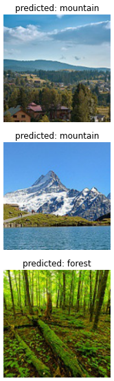
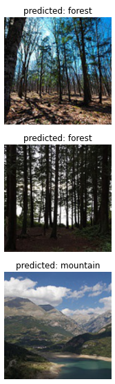


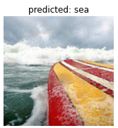

4번째 그림은 바다와 산이 같이 있기때문에 애매하긴 한데 전체적으로 잘 예측하는 것을 볼 수 있다.
ENDING
지금까지 Mobilenet v2에 대해서 알아보았다. 코랩에서 10epoch을 도는데 10분 안팎밖에 걸리지 않은 것을 보고 비록 classification이지만 이 모델이 얼마나 가벼운지 체감할 수 있었다. Object detection이나 sementic segmentation에서도 Mobilenet v2의 Inverted residual과 Linear bottleneck구조를 backbone 으로 사용하는 모델들이 많을 정도로 이 논문에서의 연산량 절감에 대한 접근이 참신하고 좋은 것 같다. Keep going..
reference
'Deep Learning' 카테고리의 다른 글
| [논문리뷰] Vision Transformer(ViT) (3) | 2021.05.15 |
|---|---|
| [논문리뷰] EfficientNet (0) | 2021.02.21 |
| [논문리뷰] YOLO v3 (0) | 2021.02.10 |
| [논문리뷰] YOLO v1 (0) | 2021.01.31 |
| Linear Regression (1) | 2021.01.26 |