논문에 대해 자세하게 다루는 글이 많기 때문에 앞으로 논문 리뷰는 모델 구현코드 위주로 작성하려고 한다.
AN IMAGE IS WORTH 16X16 WORDS: TRANSFORMERS FOR IMAGE RECOGNITION AT SCALE
Alexey Dosovitskiy∗,† , Lucas Beyer∗ , Alexander Kolesnikov∗ , Dirk Weissenborn∗ , Xiaohua Zhai∗ , Thomas Unterthiner, Mostafa Dehghani, Matthias Minderer, Georg Heigold, Sylvain Gelly, Jakob Uszkoreit, Neil Houlsby∗,† ∗ equal technical contribution, † equal advising Google Research, Brain Team
오늘은 2020년 10월에 아카이브에 등재된 구글 리서치 브레인 팀에서 발표한 Vision Transformer에 대해 알아보자.
이 논문의 중점은 NLP 분야에서 사용하고 있는 Transformer를 image classification 분야에 맞게 약간 변형하면서 기존의 CNN을 전혀 사용하지 않고 적용을 했다는 것이다.
결과적으로 당시 여러 dataset(ImageNet, ImageNet-Real, CIFAR-100)에서 SOTA 성능을 보여주면서 Transformer가 이미지 task에서 CNN기반 모델들과 비슷하거나 더 높은 성능을 보이게 된다. Transformer가 이미지 분야에 쓰이게 된게 1년이 조금 넘은 것 같은데 벌써 이정도 성능을 보이니 CNN이 더이상 쓰이지 않게 되지 않을까 라는 생각이 들기도 한다.
이런 Vision Transformer의 단점이라고 한다면 바로 학습에 필요한 데이터의 양이다.
실제로 단순히 ImageNet과 같은 규모의 데이터셋만 사용해서 학습을 하면 ResNet보다 조금 아래의 정확도를 보여준다고 한다. 그 이유는 translation equivariance 및 locality 와 같은 CNN 고유의 inductive bias(보지 못한 입력에 대한 출력을 예측할때 사용되는 가설 ex) SVM의 inductive bias는 경계와의 margin을 가장 크게 하는것)가 없기 떄문에 더 많은 데이터가 필요로 한다고 한다. 그래서 Vision Transformer는 JFT-300M(3억...)에 의해 pretrained 된 weight를 사용한다.
결국 이 모델이 이정도 성능을 낼 수 있었던 것은 구글이었기 때문이지 않을까 싶다.
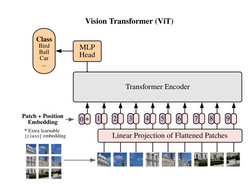
Model Architecture

Vision Transformer의 로직은 다음과 같다.
- 이미지를 여러개의 패치(base model의 patch는 16x16 크기)로 자른후에 각 패치별로 1차원 embedding demension(16x16x3 = 768)으로 만든다.
- class token이라는 것을 concatenate 시키고 각 패치마다 Position Embedding을 더해준다 (class token은 패치가 아닌 이미지 전체의 Embedding을 가지고 있다는 가정하에 최종 classification head에서 사용 / Position Embedding은 각 패치의 순서를 모델에 알려주는 역할을 한다) -> cls token과 positional embedding은 모두 학습되는 파라미터
- Transformer Encoder를 n번 수행을 한다. (base model은 12번의 block 수행) -> Layer Normalization을 사용하며 기존 바닐라 Transformer와는 다르게 Attention과 MLP이전에 수행을 하게 되면서 깊은 레이어에서도 학습이 잘 되도록 했다고 한다.
- 최종적으로 Linear연산을 통해 classification을 하게 된다.
Pytorch Implementation
1. Patch Embedding
class PatchEmbed(nn.Module):
    def __init__(self, img_size, patch_size, in_chans=3, embed_dim=768):
        super(PatchEmbed, self).__init__()
        self.img_size = img_size
        self.patch_size = patch_size
        self.n_patches = (img_size // patch_size) ** 2

        self.proj = nn.Conv2d(
            in_channels=in_chans,
            out_channels=embed_dim,
            kernel_size=patch_size,
            stride=patch_size,
        )  # Embedding dim으로 변환하며 패치크기의 커널로 패치크기만큼 이동하여 이미지를 패치로 분할 할 수 있음.

    def forward(self, x):
        x = self.proj(x)  # (batch_size, embed_dim, n_patches ** 0.5, n_patches ** 0.5)
        x = x.flatten(2)  # 세번째 차원부터 끝까지 flatten (batch_size, embed_dim, n_patches)
        x = x.transpose(1, 2)  # (batch_size, n_patches, embed_dim)
return x- 초반에 언급했지만 VIsion Transformer는 전혀 CNN을 사용하지 않는다고 하였다. 그런데 중간에 nn.Conv2d() 가 떡하니 있어 의아할 수 있다. 하지만 자세히 보면 kernerl_size와 stride가 패치 사이즈(16)로 되어 있기 때문에 서로 겹치지 않은 상태로 16x16의 패치로 나눈다는 의미로 해석할 수 있다.
- 입력 이미지 사이즈가 384x384 라고 했을때 Convolution을 수행하게 되면 차원이 (n, 768, 24, 24) 가 될 것이고 여기서 flatten과 transpose를 사용해서 (n, 576, 768)의 각 패치별(576개) 1차원 벡터(768 embed dim)로 표현 가능하다.
2. Multi Head Attention
class Attention(nn.Module):
    def __init__(self, dim, n_heads=12, qkv_bias=True, attn_p=0., proj_p=0.):
        super(Attention, self).__init__()
        self.n_heads = n_heads
        self.dim = dim
        self.head_dim = dim // n_heads
        self.scale = self.head_dim ** -0.5  # 1 / root(self.head_dim)
        '''
        # 나중에 query와 key를 곱하고 softmax를 취하기전에 scale factor로 나눠주는데 이 scale factor의 역할은
        query @ key 의 값이 커지게 되면 softmax 함수에서의 기울기 변화가 거의 없는 부분으로 가기때문에 gradient vanishing
        문제를 해결하려면 scaling을 해주어야 한다고 Attention is all you need 논문에서 주장

        '''
        self.qkv = nn.Linear(dim, dim*3, bias=qkv_bias)
        self.attn_drop = nn.Dropout(attn_p)
        self.proj = nn.Linear(dim, dim)
        self.proj_drop = nn.Dropout(proj_p)

    def forward(self, x):
        n_samples, n_tokens, dim = x.shape
        if dim != self.dim:
            raise ValueError

        qkv = self.qkv(x)  # (n_samples, n_patches+1, dim*3)
        qkv = qkv.reshape(
            n_samples, n_tokens, 3, self.n_heads, self.head_dim
        )  # (n_samples, n_patches+1, 3, n_heads, head_dim)
        qkv = qkv.permute(2, 0, 3, 1, 4)  # (3, n_samples, n_heads, n_patches+1, head_dim)
        q, k, v = qkv[0], qkv[1], qkv[2]  # 각각의 n_heads끼리 query, key, value로 나눔
        k_t = k.transpose(-2, -1)  # (n_samples, n_heads, head_dim, n_patches+1)  dot product를 위한 transpose
        # dot product를 통해 query와 key사이의 유사도를 구함
        dp = (q @ k_t) * self.scale  # (n_samples, n_heads, n_patches+1, n_patches+1)  @: dot product (2x1)@(1x2)=(2x2)
        attn = dp.softmax(dim=-1)  # attention (n_samples, n_heads, n_patches+1, n_patches+1)
        attn = self.attn_drop(attn)

        weighted_avg = attn @ v  # (n_samples, n_heads, n_patches+1, head_dim)
        # 원래 차원으로 되돌림.
        weighted_avg = weighted_avg.transpose(1, 2)  # (n_samples, n_patches+1, n_heads, head_dim)
        weighted_avg = weighted_avg.flatten(2)  # concat (n_samples, n_patches+1, dim)

        x = self.proj(weighted_avg)  # linear projection (n_samples, n_patches+1, dim)
        x = self.proj_drop(x)
return x- n_patches+1을 하는 이유는 class token을 attention 이전부터 붙이기 때문
- self.qkv 에서 dim을 3배로 키우는 이유는 query, key, value를 분할 하기 위함
- query와 key를 dot product를 하고 softmax를 취함으로써 둘의 연관성을 구한다.
- 그다음 softmax를 취하기 전에 이 attention score를 scale로 나눠주게 되는데 attention score값이 커지게 되면 softmax함수에서 기울기변화가 없는 부분으로 가기 때문에 gradient vanishing을 막기 위함이다.
- softmax를 취한후 value를 곱해 최종 attention을 구하게 된다.
- value를 곱하는 이유는 관련이 있는 단어들은 그대로 남겨두고 관련이 없는 단어들은 작은 숫자(점수)를 곱해 없애버리기 위함.
3. MLP(Multi Layer Perceptron)
class MLP(nn.Module):
    def __init__(self, in_features, hidden_features, out_features, p=0.):
        super(MLP, self).__init__()
        self.fc1 = nn.Linear(in_features, hidden_features)
        self.act = nn.GELU()
        self.fc2 = nn.Linear(hidden_features, out_features)
        self.drop = nn.Dropout(p)

    def forward(self, x):
        x = self.fc1(x)
        x = self.act(x)
        x = self.drop(x)
        x = self.fc2(x)
        x = self.drop(x)
        return x
- MLP는 아주 간단하게 hidden dimension으로 한번 갔다가 돌아오도록 되어있고 hidden dimension은 base model에서 3072로 하고있다.
- 여기서 activation으로 GELU라는 것을 사용하는데 GELU는 Gaussian Error Linear Unit의 약자이며 다른 알고리즘보다 수렴속도가 빠르다는 특징을 가지고 있다.

4. Transformer Encoder Block
class Block(nn.Module):
    def __init__(self, dim, n_heads, mlp_ratio=4.0, qkv_bias=True, p=0., attn_p=0.):
        super(Block, self).__init__()
        self.norm1 = nn.LayerNorm(dim, eps=1e-6)
        self.attn = Attention(
            dim,
            n_heads=n_heads,
            qkv_bias=qkv_bias,
            attn_p=attn_p,
            proj_p=p
        )
        self.norm2 = nn.LayerNorm(dim, eps=1e-6)
        hidden_features = int(dim * mlp_ratio)  # 3072(MLP size)
        self.mlp = MLP(
            in_features=dim,
            hidden_features= hidden_features,
            out_features=dim,
        )

    def forward(self, x):
        x = x + self.attn(self.norm1(x))
        x = x + self.mlp(self.norm2(x))
return x- Vision Transformer의 Encoder를 반복하는 block이다.
- 유의할 부분은 attention와 mlp 앞에 Layer Normalization이 먼저 수행되고 skip connection이 각각 들어가게 된다.
Layer Normalization?
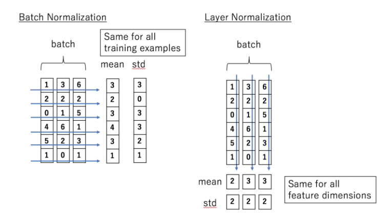

- 먼저 Batch Normalization은 N,H,W에 대해서만 연산을 진행한다. 따라서 평균과 표준편차는 channel map C와는 무관하게 계산되어 batch N에 대해 normalization 된다.
- Layer Normalization은 C,H,W에 대해서만 연산을 하므로 batch N과는 무관하게 평균과 표준편차를 구한다. 즉 channel map C에 대해 normalization 된다는 의미이다.
- LayerNorm input data가 (n, 577, 768)일때 dim방향으로 normalize가 일어 나므로 577개의 각각의 패치마다 평균과 분산이 다르게 적용되어 normalize된다.
- NLP의 Transformer를 따온 모델이기 때문에 embedding vector를 Layer Normalization 으로 사용하는 것 같다.
5. Vision Transformer
class VisionTransformer(nn.Module):
    def __init__(
            self,
            img_size=384,
            patch_size=16,
            in_chans=3,
            n_classes=1000,
            embed_dim=768,
            depth=12,
            n_heads=12,
            mlp_ratio=4.,
            qkv_bias=True,
            p=0.,
            attn_p=0.):
        super(VisionTransformer, self).__init__()

        self.patch_embed = PatchEmbed(
            img_size=img_size,
            patch_size=patch_size,
            in_chans=in_chans,
            embed_dim=embed_dim,
        )
        self.cls_token = nn.Parameter(torch.zeros(1, 1, embed_dim))
        self.pos_embed = nn.Parameter(torch.zeros(1, 1 + self.patch_embed.n_patches, embed_dim))
        self.pos_drop = nn.Dropout(p=p)

        self.blocks = nn.ModuleList(
            [
                Block(
                    dim=embed_dim,
                    n_heads=n_heads,
                    mlp_ratio=mlp_ratio,
                    qkv_bias=qkv_bias,
                    p=p,
                    attn_p=attn_p,
                )
                for _ in range(depth)  # 12개의 block
            ]
        )

        self.norm = nn.LayerNorm(embed_dim, eps=1e-6)
        self.head = nn.Linear(embed_dim, n_classes)

    def forward(self, x):
        n_samples = x.shape[0]
        x = self.patch_embed(x)  # (n_samples, n_patches, embed_dim)
        cls_token = self.cls_token.expand(n_samples, -1, -1)  # (n_samples, 1, embed_dim)
        x = torch.cat((cls_token, x), dim=1)  # (n_samples, 1+n_patches, embed_dim)
        x = x + self.pos_embed  # (n_samples, 1+n_patches, embed_dim)
        x = self.pos_drop(x)

        for block in self.blocks:
            x = block(x)  # (n_samples, 577, 768)

        x = self.norm(x)

        cls_token_final = x[:, 0]  # just tje CLS token
        x = self.head(cls_token_final)

        return x
- 최종 Vision Transformer 구조를 구축하는 class이다.
- 처음 이미지가 들어오게 되면 self.patch_embed를 통해 (n, 576, 768)으로 만들고 class token을 패치 개수 차원으로 더해주고 position embedding을 더해준다. 이때 nn.Parameter를 통해 class token과 position embedding이 0으로 초기화가 되는데 patch embedding과는 별개로 따로 학습되는 레이어라고 생각하면 될 것같다.
- 그 다음 block의 개수만큼 Encoding이 반복수행된다. 이때 class token이 추가되면서 패치의 개수가 576개에서 577개로 1개 증가한 것을 알 수 있고 Encoder의 입력과 출력 차원이 똑같기 때문에 block이 여러번 수행될수 있다.
- Encoder 연산이 끝나게 되면 LayerNorm을 한번 수행하고 class token만 따로 추출해서 거기서 classifier를 수행하게 된다. 그 이유는 앞서 말한것 처럼 class token이 이미지 전체의 embedding을 표현하고 있음을 가정하기 때문이다.
- 최종 출력으로 Dataset class수에 맞게 값이 나오고 여기서 최대값이 예측값이 된다. (n_sanples, n_classes)
6. Model Output
if __name__ == '__main__':
    from torchsummary import summary

    custom_config = {
        "img_size": 384,
        "in_chans": 3,
        "patch_size": 16,
        "embed_dim": 768,
        "depth": 12,
        "n_heads": 12,
        "qkv_bias": True,
        "mlp_ratio": 4
    }
    model_custom = VisionTransformer(**custom_config)

    inp = torch.rand(2, 3, 384, 384)
    res_c = model_custom(inp)
    print(res_c.shape)

    summary(model_custom, input_size=(3, 384, 384), device='cpu')
    print(model_custom)
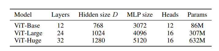
- base model 파라미터 수 : 86,415,592(86M)
- pretrained model은 timm 모듈을 사용해서 받을 수 있다.
- model_official = timm.create_model('vit_base_patch16_384', pretrained=True)
- 모델 이름은 print(timm.list_models('vit*'))를 통해 vision_transformer의 모델만 확인할 수 있다.
7. Pretrained model inference
import numpy as np
from PIL import Image
import torch.nn.functional
import cv2

k = 10  # 상위 10개

imagenet_labels = dict(enumerate(open("classes.txt")))  # ImageNet 1000 classes

model = torch.load("vit.pth")  # timm Pretrained model
model.eval()


img = (np.array(Image.open("cat.jpg"))/128) - 1  # -1~1
img = cv2.resize(img, (384, 384))
inp = torch.from_numpy(img).permute(2, 0, 1).unsqueeze(0).to(torch.float32)
logits = model(inp)
probs = torch.nn.functional.softmax(logits, dim=1)

top_probs, top_idxs = probs[0].topk(k)

for i, (idx_, prob_) in enumerate(zip(top_idxs, top_probs)):
    idx = idx_.item()
    prob = prob_.item()
    cls = imagenet_labels[idx].strip()
    print(f"{i}: {cls:<45} --- {prob:.4f}")
0: tabby, tabby_cat --- 0.9003
1: tiger_cat --- 0.0705
2: Egyptian_cat --- 0.0267
3: lynx, catamount --- 0.0013
4: Persian_cat --- 0.0002
5: Siamese_cat, Siamese --- 0.0001
6: tiger, Panthera_tigris --- 0.0000
7: snow_leopard, ounce, Panthera_uncia --- 0.0000
8: cougar, puma, catamount, mountain_lion, painter, panther, Felis_concolor --- 0.0000
9: lens_cap, lens_cover --- 0.0000
Ending
오늘은 Vision Transformer에 대해 정리해보았다. 항상 CNN중심 모델을 보다가 NLP에서 넘어온 Transformer의 구조를 보니까 너무 어색했고 이해가 잘 안되서 여러번 반복학습 했다. NLP 분야에서 사용되던 것이 이미지 분야에서 재활용 되는것을 보니까 비전 분야만 공부할 것이 아니라 다른 분야도 한번씩 둘러보면서 새로운 아이디어를 얻거나 이미지 분야로의 재활용 가능성을 고민해보면 좋을 것 같다.
Keep going
Reference
- Paper - https://arxiv.org/abs/2010.11929
- Implementation - https://www.youtube.com/watch?v=ovB0ddFtzzA&t=2s
'Deep Learning' 카테고리의 다른 글
| [논문리뷰] MLP-Mixer (0) | 2021.05.18 |
|---|---|
| Test Time Augmentation(TTA) (0) | 2021.05.17 |
| [논문리뷰] EfficientNet (0) | 2021.02.21 |
| [논문리뷰] Mobilenet v2 (0) | 2021.02.14 |
| [논문리뷰] YOLO v3 (0) | 2021.02.10 |